Table of Contents

1. Overview
2. Surveys
   1. Neural Architecture Search: A Survey
      1. Search Space
         1. Chain-Structured Search Space
         2. Chain-Structured with Skips
         3. Segment-based
      2. Cell-based Structure
      3. Search Strategy
         1. Reinforcement Learning Strategy
         2. Neron-Evolutionary Strategy
         3. Gradient-based Optimization
      4. Performance Estimation Strategy
      5. Future Directions
3. Paper Summary
   1. MnasNet: Platform-Aware Neural Architecture Search for Mobile
   2. Once-For-All: Train One Network and Specialize It For Efficient Deployment
      1. Motivation
      2. Contributions
   3. Black Box Search Space Profiling for Accelerator-Aware Neural Architecture Search
      1. Motivation
      2. Contribution
         1. The Complete NAS Workflow
         2. How to Optimize Search Space?
         3. How to Correct Block Latency?

Overview

Neural Architecture Search, or NAS, can be seen as a subtask of AutoML. It tries to automate the designing process of neural network architectures. An architecture search space can be seen as a Directed Asyclic Graph (DAG), and each possible architecture is a subgraph. We denote the search space as $A$, the subgraph $a$, the searched neural network $N(a,w)$. The goals of NAS are often two-fold:

• Weight Optimization

$$w_a = \underset{w}{\operatorname{argmin}}(Loss_{train}(N(a,w)))$$

• Architecture Optimization

$$a^* = \underset{a\in A}{\operatorname{argmax}}(Accuracy_{val}(N(a,w)))$$

The constraints are diverse: such as computation (FLOPS), speed (latency), or even energy consumption and memory usage.

Surveys

Neural Architecture Search: A Survey

• Authors: Thomas Elsken, Jan Hendrik Metzen, Frank Hutter
• Institution: Bosch Center for AI, University of Freiburg
• arXiv: https://arxiv.org/abs/1808.05377

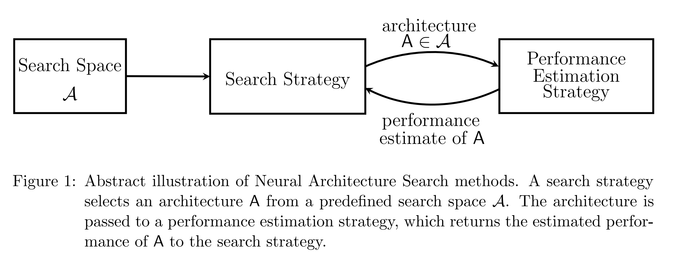
NAS methods encompasses three sub-tasks: designing search space, select search strategy, and use proper estimation strategy.

Search Space

The search space defines what architectures are discoverable during search. Search space designs can be largely classified into global search space and cell-based search space.

• Global: chain-structured, chain-structured with skip, segment-based
• Cell-based

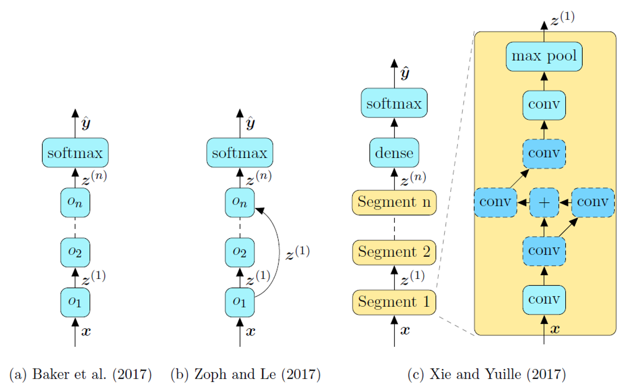
Chain-Structured Search Space

The simplist form of search space. Parameters include: the number of layers, the type of layers, hyperparameters of the layers, e.g., number of filters, kernel sizes and strides for convolutional layer.

Chain-Structured with Skips

Obviously the idea comes from ResNet, DenseNet or Xception. The branching can be described with layer’s inputs as a function

$$g_i (L_{i-1}^{out}, ..., L_0^{out})$$

Taking existing architectures for example, for chain-structured net, $g_i (L_{i-1}^{out}, ..., L_0^{out}) = L_{i-1}^{out}$. For ResNet, $g_i (L_{i-1}^{out}, ..., L_0^{out}) = L_{i-1}^{out} + L_j^{out}, (j < i-1)$. For DenseNet, $g_i (L_{i-1}^{out}, ..., L_0^{out}) = concat(L_{i-1}^{out},...,L_0^{out})$

Segment-based

Segment-based method is considered as a global search space design, but with another level of granularity: segment, or block.

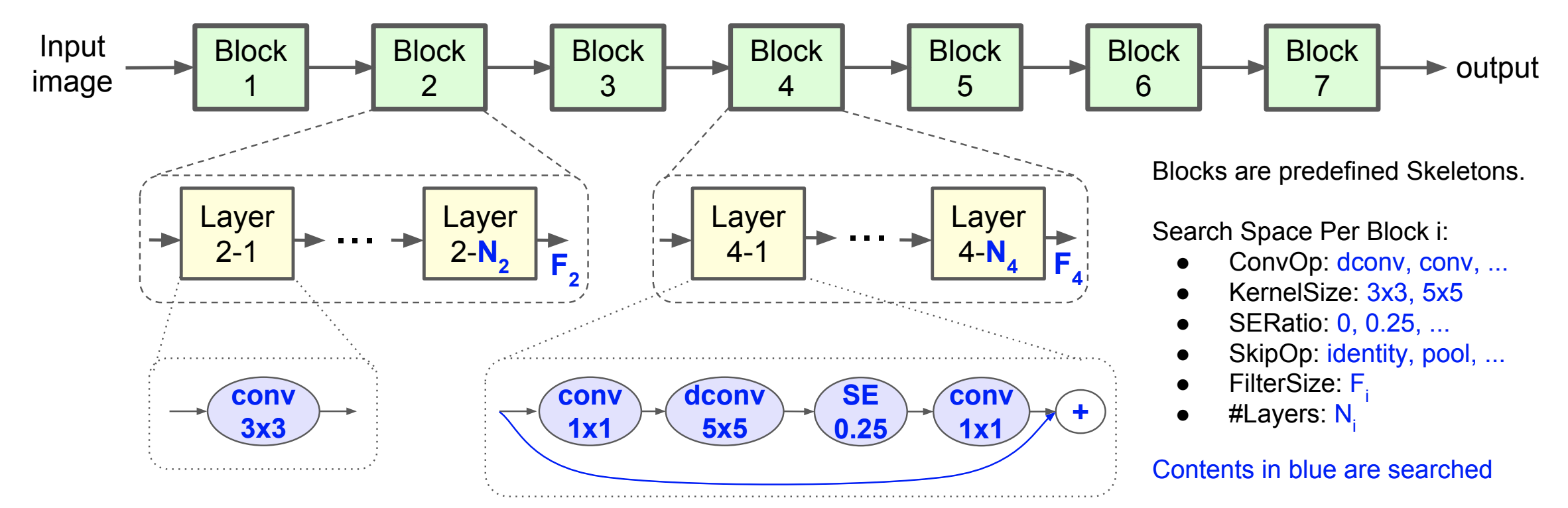
Taking Mnas as an example, the network layers are grouped into a many blocks. The skeleton constructed with blocks is predefined. Inside each block, there are a variable number of repeated layers. Blocks are not necessarily the the same, the layer amount and operations can be different.

Cell-based Structure

Cell-based architecture is a lot like the segment-based one. However, instead of searching the topology/hyperparameters of each block, cell-based approach defines several types of cells, then connects repeated cells in a pre-defined manner. In such ways, the search space is further downsized.

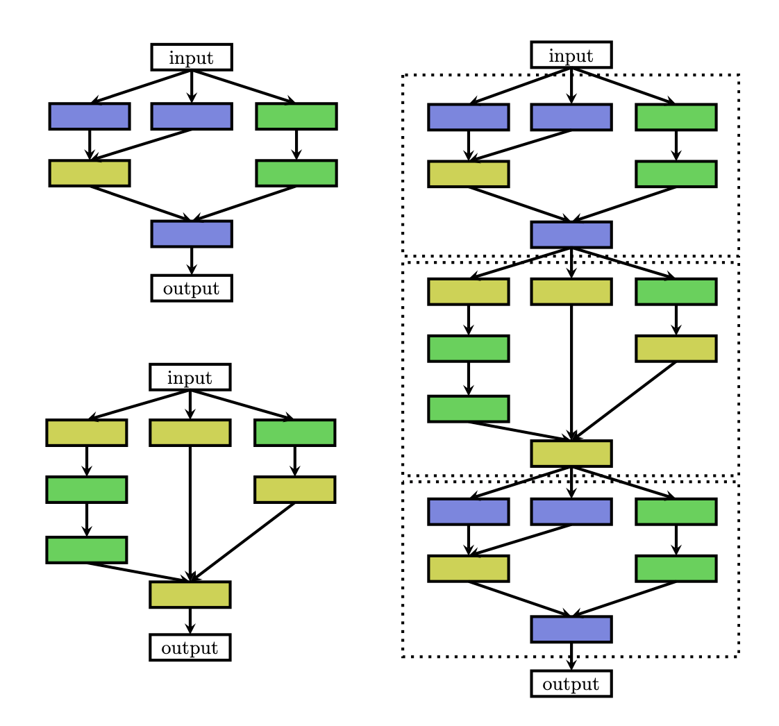
(Zoph, 2018) defined two types of cell: normal cell or reduction cell. Normal cell preserves dimensionality while reduction cell reduces spatial dimensions.

The problem of cell-based structure is that the macro-architecture, i.e. the structure based on cells, are still manually designed. (Liu, 2018b) tried to overcome macro-architecture engineering by introducing hierarchical search space.

Search Strategy

Reinforcement Learning Strategy

Different RL approaches differ in how they represent the agent’s policy and how they optimize it.

• Architecture generation: agent’s action
• Search space: action space
• Evaluation: agent’s reward is based on an estimate of the performance.

Agent’s Policy:

• RNN policy: sequentially sample a string that encodes the architecture
• …

Training method:

• REINFORCE policy gradient algorithm
• Proximal Policy Optimization
• Q-learning

Neron-Evolutionary Strategy

Neuro-evolutionary methods differ in how they sample parents, udpate populations, and generate offsprings.

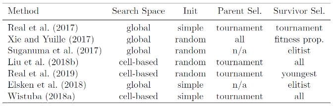
In the context of NAS, mutations are local operations, such as adding or removing a layer, altering the hyperparameters of a layer, adding skip connections.

Gradient-based Optimization

(Liu, 2019b) proposed a continuous relaxation to enable direct gradient-based optimization: instead of fixing a single operation $o_i$ to be executed at a specific layer, the authors compute a convex combination from a set of operations ${o_1, ..., o_m}$. Given a layer input $x$, the layer output $y$ is computed as $y = \sum_{i=1}^m \alpha_i o_i(x)$, $(\alpha_i \geq 0, \sum_{i=1}^m \alpha_i = 1)$

Performance Estimation Strategy

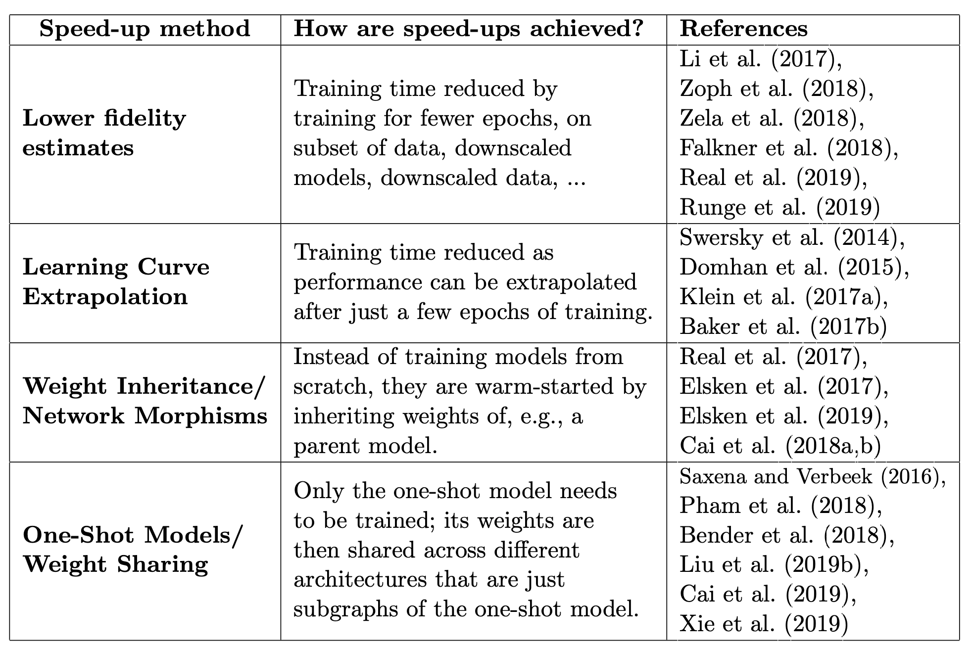
• Lower Fidelity
  The bias in the estimation is the gap between the full evaluation. This may not be problematic as only relative ranking is considered. But when the gap is large, the relative ranking may not be stable.

• Learning Curve Extrapolation or Surrogate Model
  Using early learning curve of architecture information to extrapolate performance.

• Network Morphism
  No inherent search space upper bound. However, strict netwrok morphisms can only make architectures larger, therefore leading to redundancy.

• One-Shot
  Training only one supernet, so only validation is needed at evaluation stage. The supernet restricts the search space, and may be limited by GPU memory.

  • ENAS learns a RNN controller that samples architectures from the search space and trains the one-shot model based on approximate gradients obtained through REINFORCE.
  • DARTS jointly optimize all weights with a continuous relaxation of the search space.
  • SNAS optimizes a distribution over the candidate operations. The authors employ the concrete distribution and reparameterization to relax the discrete distribution and make it differentiable.
  • Proxyless NAS “binarizes” the weights, maksing out all but one edge per operation to overcome the necessity of keeping the entire supernet model in GPU memory.

It is currently not well understood which biases they introduce into the search if the sampling of distribution of architectures is optimized along with the one-shot model instead of fixing it. For example, an initial bias in exploring certain parts of the search space more than others might lead to the weights of the one-shot model being better adapted for these architectures, which in turn would reinforce the bias of the search to these parts in the search space. This might result in premature convergence of NAS or little correlation between the one-shot and true performance of an architecture.

Future Directions

1. Applying NAS to less explored domains, such as image restoration, semantic segmentation, transfer learning, machine translation, GAN, or sensor fusion.
2. Develop MAS methos for multi-task problems, and for multi-objective problems, such as latency and power optimization.
3. Universal NAS on different tasks. More general and flexible search space design.
4. Developing benchmarks.

While NAS has achieved impressive performance, so far it provides little insights into why specific architectures work well and how similar the architectures derived in indepen- dent runs would be. Identifying common motifs, providing an understanding why those motifs are important for high performance, and investigating if these motifs generalize over different problems would be desirable.

Paper Summary

MnasNet: Platform-Aware Neural Architecture Search for Mobile

• Authors: Mingxing Tan, Bo Chen et al.
• Year:
• Intitution: Google
• arXiv: https://arxiv.org/pdf/1807.11626.pdf

Once-For-All: Train One Network and Specialize It For Efficient Deployment

• Authors: Han Cai, Chuang Gan, Tianzhe Wang, Zhekai Zhang, Song Han
• Venue: ICLR 2020
• Institution: MIT
• arXiv: https://arxiv.org/abs/1908.09791
• Code: https://github.com/mit-han-lab/once-for-all

Motivation

Designing a once-for-all network that flexibly supports different depths, widths, kernel sizes, and resolutions without retraining.

Contributions

• The model training stage and architecture search stage is decoupled.
• A progressive shrinking method to trian the supernet

Black Box Search Space Profiling for Accelerator-Aware Neural Architecture Search

• Authors: Shulin Zeng, Hanbo Sun, Yu Xing, Xuefei Ning, Yi Shan, Xiaoming Chen, Yu Wang, Huazhong Yang
• Venue: 2020 ASP-DAC
• Institution: Tsinghua University, and Institute of Computing Technology, Chinese Academy of Sciences
• Xplore: https://ieeexplore.ieee.org/document/9045179

Motivation

1. Designing a suitable search space for DNN accelerators is still challenging.
2. Evaluating latency across platforms with various architectures and compilers is hard because we don’t have prior knowlege of the hardware & compiler.

Contribution

1. A black-box search space tuning method for Instruction Set Architecture (ISA) accelerators.
2. A layer-adaptive latency correction method.

The Complete NAS Workflow

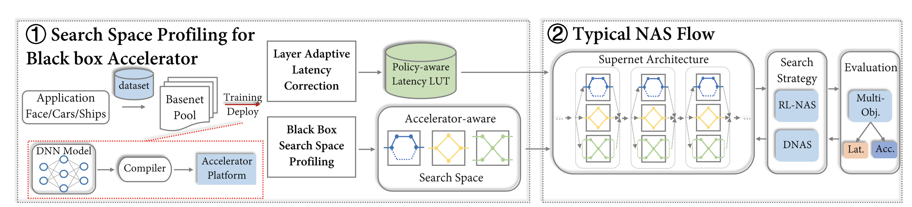
The magic happens in “Basenet Pool” and “Policy-aware Latency”, where the authors constructs a automatic search space design method. “Policy-aware Latency LUT” stands for an improved latency profiling method. Previous works use standalone block latency to build a LUT, ignoring inter-layer latency influences. Such influences are caused by compiler policies, such as “layer fusion” that combines layers to shorten latency. This new latency profiling method aims to take inter-layer latency dependencies into account without knowing the underlying compiler or hardware.

How to Optimize Search Space?

SSBN: stands for Search Space Base Network. Based on a specific net from the Search Space, change at most one block at a time to get a SSBN. Because the original Search Space can be regarded as linear combination of SSBNs, this reduces complexity without harming degree of freedom.

Generating Basenet Pool: there are currently 3 types of mainstream hand-designed blocks: VGG, Res, and MobileNet-based. For each type the authors construct a Specified Network (SN), and obtain its SSBNs. All SSBNs together are the Basenet Pool.

Selecting Search Space: for each group of SSBNs, the authors design a cost function combining accuracy and latency. For each group of SSBNs, their costs are first calculated. After that, they are sorted in ascending w.r.t. the cost. A threshold defined by the user selects a range of
SSBNs that goes into the new search space. The new search space is much smaller.

How to Correct Block Latency?

The authors design two methods for latency correction. The first one uses overall network latency measurements to calculate the difference between standalone and actual block latency. The second one is a refinement of the first. It takes other block’s latency into account, thus more fine-grained.

$$L_{BNblock}(n,l) = L_{BN}(n,l) - L_{SN} + L_{SNblock}(l)$$

• $L_{BNblock}(n,l)$ is the block latency we want to know.
• $n$ is the type of block. $l$ is the index of layer.
• $L_{SNblock}(l)$ is the standalone layer latency.
• $L_{SN}$ is the overal latency of the network.
• $L_{BN}(n,l)$ is the overall latency where the target block is substituted.

$$L_{CNblock}(n,l) = \frac{1}{L} \sum_{(n',l' \in CN)} L_{BNblock}(n, l, n')$$

This one is difficult to understand.

$L$ is the number of layers (or blocks) in the network. The authors first create $L$ networks preserving the target block but the rest are all one particular type. Then within each of these “Specified Network”, our target block’s latency is measured with method 1. At last, the block latency measurements are averaged to get the estimated “candidate network (CN)” block latency.